Table of Contents

• 1  Dataset introduction

  • 1.1  Data loading

    • 1.1.1  Access to internal DataFrame

    • 1.1.2  Access to numerical/categorical variables

    • 1.1.3  Set the target variable

    • 1.1.4  Access to features

  • 1.2  Data description

  • 1.3  Data Maniuplation

    • 1.3.1  Remove columns

    • 1.3.2  Add columns

    • 1.3.3  Remove samples

    • 1.3.4  Samples Matching criteria

  • 1.4  Data Conversion

    • 1.4.1  Type conversion (int, float)

    • -Numerical” data-toc-modified-id=”Categorical-<->-Numerical-1.4.2”>1.4.2  Categorical <-> Numerical

• 2  Histograms and density plots

  • 2.1  Histograms

  • 2.2  Density plots

  • 2.3  Features importance

  • 2.4  Covariance Matrix

  • 2.5  Native pandas plots

• 3  Data cleaning

  • 3.1  NA’s

    • 3.1.1  Replace NA

  • 3.2  Outliers

  • 3.3  Correlation

  • 3.4  Under represented features

    • 3.4.1  Merge categories

    • 3.4.2  Merge values

• 4  Data transformation

  • 4.1  One-hot encoding

  • 4.2  Discretize

  • 4.3  Skewness

  • 4.4  Scale

• 5  Feature selection

  • 5.1  Information Gain

  • 5.2  Stepwise feature selection

• 6  Dataset Split

from dataset import Dataset
import numpy as np
import matplotlib.pyplot as plt

Dataset introduction

The idea with Dataset is that you simplify most of the tasks that you normally do with pandas DataFrame. This normally applies when you’re starting in Python. You will have access at any time, to the underlying pandas DataFrame that holds the data, in case you need to use the numpy representation of the values, or access specific locations of your data.

Data loading

To start with Dataset, you must load your data the same way it is done with pandas, by passing the URL or file location to the constructor (Dataset()). If you need to add more pandas parameters to this call, specifying what is the separator, or whether to use headers, etc., simply add them after the file location.

I’m using the location of the CSV from U.Arizona.

URL="https://www2.cs.arizona.edu/classes/cs120/fall17/ASSIGNMENTS/assg02/Pokemon.csv"
pokemon = Dataset(URL, delimiter=',', header=0)

From this point, you have access to the methods provided by Dataset to describe the dataset, clean up your data, perform feature selection or plot some interesting feature engineering related plots.

If you already have a DataFrame and want to use inside a Dataset class, you can also import it, using the method:

>>> my_dataset = Dataset.from_dataframe(my_dataframe)

 Access to internal DataFrame

If you want access your DataFrame you simply have to call the property features at the end of the Dataset name:

pokemon.features

	#	Name	Type 1	Type 2	Total	HP	Attack	Defense	Sp. Atk	Sp. Def	Speed	Generation	Legendary
0	1.0	Bulbasaur	Grass	Poison	318.0	45.0	49.0	49.0	65.0	65.0	45.0	1.0	False
1	2.0	Ivysaur	Grass	Poison	405.0	60.0	62.0	63.0	80.0	80.0	60.0	1.0	False
2	3.0	Venusaur	Grass	Poison	525.0	80.0	82.0	83.0	100.0	100.0	80.0	1.0	False
3	3.0	VenusaurMega Venusaur	Grass	Poison	625.0	80.0	100.0	123.0	122.0	120.0	80.0	1.0	False
4	4.0	Charmander	Fire	NaN	309.0	39.0	52.0	43.0	60.0	50.0	65.0	1.0	False
...	...	...	...	...	...	...	...	...	...	...	...	...	...
795	719.0	Diancie	Rock	Fairy	600.0	50.0	100.0	150.0	100.0	150.0	50.0	6.0	True
796	719.0	DiancieMega Diancie	Rock	Fairy	700.0	50.0	160.0	110.0	160.0	110.0	110.0	6.0	True
797	720.0	HoopaHoopa Confined	Psychic	Ghost	600.0	80.0	110.0	60.0	150.0	130.0	70.0	6.0	True
798	720.0	HoopaHoopa Unbound	Psychic	Dark	680.0	80.0	160.0	60.0	170.0	130.0	80.0	6.0	True
799	721.0	Volcanion	Fire	Water	600.0	80.0	110.0	120.0	130.0	90.0	70.0	6.0	True

800 rows × 13 columns

If, instead of displaying the entire pandas DataFrame we want to see a special feature, we can refer to that feature using its name, right after the features property. In this case, let’s have a look to the feature called Name holding the pokemon name.

pokemon.features.Name

0                  Bulbasaur
1                    Ivysaur
2                   Venusaur
3      VenusaurMega Venusaur
4                 Charmander
               ...
795                  Diancie
796      DiancieMega Diancie
797      HoopaHoopa Confined
798       HoopaHoopa Unbound
799                Volcanion
Name: Name, Length: 800, dtype: object

The result from this call is pandas Series.

or (to show only the first 5 lines from the dataframe):

pokemon.features.head(3)

	#	Name	Type 1	Type 2	Total	HP	Attack	Defense	Sp. Atk	Sp. Def	Speed	Generation	Legendary
0	1.0	Bulbasaur	Grass	Poison	318.0	45.0	49.0	49.0	65.0	65.0	45.0	1.0	False
1	2.0	Ivysaur	Grass	Poison	405.0	60.0	62.0	63.0	80.0	80.0	60.0	1.0	False
2	3.0	Venusaur	Grass	Poison	525.0	80.0	82.0	83.0	100.0	100.0	80.0	1.0	False

Number of features and number of samples in the dataset are accessible through the following properties:

print('Nr of features:', pokemon.num_features)
print('Nr of samples:', pokemon.num_samples)

Nr of features: 13
Nr of samples: 800

Access to numerical/categorical variables

It is also possible to work only with the numerical or categorical variables in the dataset. To do that you just have to use the properties: .categorical or .numerical to access those portions of the dataframe that only contain those feature subtypes.

If we want to access only the categorical, we type:

pokemon.categorical.head(3)

	Name	Type 1	Type 2	Legendary
0	Bulbasaur	Grass	Poison	False
1	Ivysaur	Grass	Poison	False
2	Venusaur	Grass	Poison	False

If we want to access the numerical ones:

pokemon.numerical.head(3)

	#	Total	HP	Attack	Defense	Sp. Atk	Sp. Def	Speed	Generation
0	1.0	318.0	45.0	49.0	49.0	65.0	65.0	45.0	1.0
1	2.0	405.0	60.0	62.0	63.0	80.0	80.0	60.0	1.0
2	3.0	525.0	80.0	82.0	83.0	100.0	100.0	80.0	1.0

In case we want only the names of the variables that are numerical or categorical, we can either use:

pokemon.categorical_features

['Name', 'Type 1', 'Type 2', 'Legendary']

or

pokemon.names('categorical')

['Name', 'Type 1', 'Type 2', 'Legendary']

which, of course, also applies to numerical.

Set the target variable

At this point, we can make something very interesting when working with datasets, which is to select what feature will be the target variable. By doing so, Dataset will separate that feature from the rest, allowing to use special feature engineering methods that we will se afterwards:

pokemon.set_target('Legendary');

When we select the target, that feature dissapears from the features property, as you can see when we call the head method again:

pokemon.features.head(3)

	#	Name	Type 1	Type 2	Total	HP	Attack	Defense	Sp. Atk	Sp. Def	Speed	Generation
0	1.0	Bulbasaur	Grass	Poison	318.0	45.0	49.0	49.0	65.0	65.0	45.0	1.0
1	2.0	Ivysaur	Grass	Poison	405.0	60.0	62.0	63.0	80.0	80.0	60.0	1.0
2	3.0	Venusaur	Grass	Poison	525.0	80.0	82.0	83.0	100.0	100.0	80.0	1.0

Our feature is now in a new property called target. We cann access it, by calling it from our Dataset, which will return a pandas Series object to work with.

pokemon.target

0      False
1      False
2      False
3      False
4      False
       ...
795     True
796     True
797     True
798     True
799     True
Name: Legendary, Length: 800, dtype: bool

If at any point during your work you want to unset the target variable, and make it part of the dataset again as a normal feature, you just have to call

>>> pokemon.unset_target()

From that point, no target variable is defined within the dataset and all features are considered normal features.

Access to features

From this point, if we want to access a DataFrame that will contain all features, including the target variable, we must use the property all, because, as you can see, features no longer contains the target variable:

pokemon.all.head(3)

	#	Name	Type 1	Type 2	Total	HP	Attack	Defense	Sp. Atk	Sp. Def	Speed	Generation	Legendary
0	1.0	Bulbasaur	Grass	Poison	318.0	45.0	49.0	49.0	65.0	65.0	45.0	1.0	False
1	2.0	Ivysaur	Grass	Poison	405.0	60.0	62.0	63.0	80.0	80.0	60.0	1.0	False
2	3.0	Venusaur	Grass	Poison	525.0	80.0	82.0	83.0	100.0	100.0	80.0	1.0	False

Data description

First thing we can do with our dataset is to describe it, just to know the types of the variables, and whether we have NA’a or incomplete features.

pokemon.describe()

12 Features. 800 Samples
Available types: [dtype('float64') dtype('O')]
  · 3 categorical features
  · 9 numerical features
  · 1 categorical features with NAs
  · 0 numerical features with NAs
  · 12 Complete features
--
Target: Legendary (bool)
'Legendary'
  · Min.: 0.0000
  · 1stQ: 0.0000
  · Med.: 0.0000
  · Mean: 0.0813
  · 3rdQ: 0.0000
  · Max.: 1.0000

In case you want more information about the values, each feature is taking, then you can use the summary() method:

pokemon.summary()

Features Summary (all):
'#'         : float64    Min.(1.0) 1stQ(184.) Med.(364.) Mean(362.) 3rdQ(539.) Max.(721.)
'Name'      : object     800 categs. 'Bulbasaur'(1, 0.0013) 'Ivysaur'(1, 0.0013) 'Venusaur'(1, 0.0013) 'VenusaurMega Venusaur'(1, 0.0013) ...
'Type 1'    : object     18 categs. 'Grass'(112, 0.1400) 'Fire'(98, 0.1225) 'Water'(70, 0.0875) 'Bug'(69, 0.0862) ...
'Type 2'    : object     18 categs. 'Poison'(97, 0.2343) 'nan'(35, 0.0845) 'Flying'(34, 0.0821) 'Dragon'(33, 0.0797) ...
'Total'     : float64    Min.(180.) 1stQ(330.) Med.(450.) Mean(435.) 3rdQ(515.) Max.(780.)
'HP'        : float64    Min.(1.0) 1stQ(50.0) Med.(65.0) Mean(69.2) 3rdQ(80.0) Max.(255.)
'Attack'    : float64    Min.(5.0) 1stQ(55.0) Med.(75.0) Mean(79.0) 3rdQ(100.) Max.(190.)
'Defense'   : float64    Min.(5.0) 1stQ(50.0) Med.(70.0) Mean(73.8) 3rdQ(90.0) Max.(230.)
'Sp. Atk'   : float64    Min.(10.0) 1stQ(49.7) Med.(65.0) Mean(72.8) 3rdQ(95.0) Max.(194.)
'Sp. Def'   : float64    Min.(20.0) 1stQ(50.0) Med.(70.0) Mean(71.9) 3rdQ(90.0) Max.(230.)
'Speed'     : float64    Min.(5.0) 1stQ(45.0) Med.(65.0) Mean(68.2) 3rdQ(90.0) Max.(180.)
'Generation': float64    Min.(1.0) 1stQ(2.0) Med.(3.0) Mean(3.32) 3rdQ(5.0) Max.(6.0)
'Legendary' : bool       2 categs. 'False'(735, 0.9187) 'True'(65, 0.0813)

Data Maniuplation

Remove columns

You can easily remove columns from data by using the method drop_columns(). You can pass a single column/feature name or a list of features, and they will dissapear from the dataset.

pokemon.drop_columns('#')

<dataset.dataset.Dataset at 0x133a668d0>

You can also remove all the columns that are not in a list. To do that, you use keep_columns() and what you must pass to the function is a feature name or a list of feature names you want to keep in your dataset. For example, if we might want to keep only the numerical features:

pokemon.keep_columns(pokemon.numerical_features)

or if we might want to keep only a couple of well known features:

pokemon.keep_columns(['Total', 'Attack'])

Add columns

You can also add columns or entire dataframes to your existing dataset. If you want to simply add a pandas Series to the existing dataset, call:

pokemon.add_colums(my_data_series)

If what you want is to add an entire dataframe, the mechanism is exactly the same:

pokemon.add_columns(my_dataframe)

In the following cells, all features are shown, then categoricals are extracted to variable categoricals, and removed from the dataset. Then categoricals is added to the original dataset, resulting in a dataset which is equivalent to the one we stsarted with.

# Original dataset
pokemon.features.head(3)

	Name	Type 1	Type 2	Total	HP	Attack	Defense	Sp. Atk	Sp. Def	Speed	Generation
0	Bulbasaur	Grass	Poison	318.0	45.0	49.0	49.0	65.0	65.0	45.0	1.0
1	Ivysaur	Grass	Poison	405.0	60.0	62.0	63.0	80.0	80.0	60.0	1.0
2	Venusaur	Grass	Poison	525.0	80.0	82.0	83.0	100.0	100.0	80.0	1.0

categoricals = pokemon.categorical

pokemon.drop_columns(pokemon.categorical_features)
pokemon.features.head(3)

	Total	HP	Attack	Defense	Sp. Atk	Sp. Def	Speed	Generation
0	318.0	45.0	49.0	49.0	65.0	65.0	45.0	1.0
1	405.0	60.0	62.0	63.0	80.0	80.0	60.0	1.0
2	525.0	80.0	82.0	83.0	100.0	100.0	80.0	1.0

pokemon.add_columns(categoricals)
pokemon.features.head(3)

	Total	HP	Attack	Defense	Sp. Atk	Sp. Def	Speed	Generation	Name	Type 1	Type 2
0	318.0	45.0	49.0	49.0	65.0	65.0	45.0	1.0	Bulbasaur	Grass	Poison
1	405.0	60.0	62.0	63.0	80.0	80.0	60.0	1.0	Ivysaur	Grass	Poison
2	525.0	80.0	82.0	83.0	100.0	100.0	80.0	1.0	Venusaur	Grass	Poison

Remove samples

If what you want is to remove some samples (rows) from the dataset, you simply call the method drop_samples() passing the list of indices you want to remove. For example:

pokemon.drop_samples([34, 56, 78])

Samples Matching criteria

If you want to select samples for which one of the features fulfills a certain criteria, you can get the list of indices of those samples by calling:

print('There are', len(pokemon.samples_matching('Grass', 'Type 1')),
      'samples for which \'Type 1\' is valued \'Grass\'')

There are 70 samples for which 'Type 1' is valued 'Grass'

Data Conversion

Conversion of data in Dataset is primarily between types for numerical features (int <-> float), and between categorical and numerical, and viceversa.

 Type conversion (int, float)

To convert between float and int:

pokemon.to_int('this_is_a_float_feature')

or

pokemon.to_float(['int_feature_1', 'int_feature_2'])

Again, you can pass a single name or a list of names between brackets.

Categorical <-> Numerical

We can also convert numerical features to categorical and viceversa (when it makes sense), using:

pokemon.to_categorical('my_numerical_feature')

or

pokemon.to_numerical('my_categorical_feature')

In our case, it seems that the feature Generation could be considered as categorical. So, to convert it as a category, we better convert it first to int, to later convert it to a category. We can call both methods in the same line. We should also convert the target variable to the categorical type, since bool is often interpreted as a number (0/1).

pokemon.to_int('Generation').to_categorical(['Generation'])
pokemon.summary()

Features Summary (all):
'Total'     : float64    Min.(180.) 1stQ(330.) Med.(450.) Mean(435.) 3rdQ(515.) Max.(780.)
'HP'        : float64    Min.(1.0) 1stQ(50.0) Med.(65.0) Mean(69.2) 3rdQ(80.0) Max.(255.)
'Attack'    : float64    Min.(5.0) 1stQ(55.0) Med.(75.0) Mean(79.0) 3rdQ(100.) Max.(190.)
'Defense'   : float64    Min.(5.0) 1stQ(50.0) Med.(70.0) Mean(73.8) 3rdQ(90.0) Max.(230.)
'Sp. Atk'   : float64    Min.(10.0) 1stQ(49.7) Med.(65.0) Mean(72.8) 3rdQ(95.0) Max.(194.)
'Sp. Def'   : float64    Min.(20.0) 1stQ(50.0) Med.(70.0) Mean(71.9) 3rdQ(90.0) Max.(230.)
'Speed'     : float64    Min.(5.0) 1stQ(45.0) Med.(65.0) Mean(68.2) 3rdQ(90.0) Max.(180.)
'Generation': object     6 categs. '1'(166, 0.2075) '2'(165, 0.2062) '3'(160, 0.2000) '4'(121, 0.1512) ...
'Name'      : object     800 categs. 'Bulbasaur'(1, 0.0013) 'Ivysaur'(1, 0.0013) 'Venusaur'(1, 0.0013) 'VenusaurMega Venusaur'(1, 0.0013) ...
'Type 1'    : object     18 categs. 'Grass'(112, 0.1400) 'Fire'(98, 0.1225) 'Water'(70, 0.0875) 'Bug'(69, 0.0862) ...
'Type 2'    : object     18 categs. 'Poison'(97, 0.2343) 'nan'(35, 0.0845) 'Flying'(34, 0.0821) 'Dragon'(33, 0.0797) ...
'Legendary' : bool       2 categs. 'False'(735, 0.9187) 'True'(65, 0.0813)

Histograms and density plots

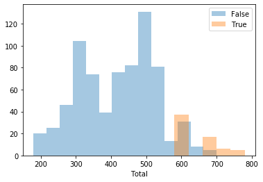
Histograms

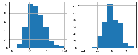
This function helps you to plot double histograms to compare feature-distributions for all possible target values. So, you must set the target variable before calling this method, or provide the name of the variable you want to compare your distribution against.

You can plot the histogram of any of the numerical variables with respect to the target variable to see what is its distribution, using (in this case we’re plotting a feature called Total against the target variable –a binomial boolean feature previsouly set):

pokemon.plot_histogram('Total')

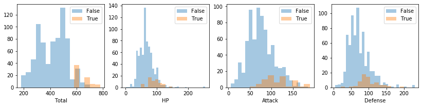
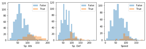
Or if you want, plot every numerical feature histogram):

pokemon.plot_histogram(pokemon.numerical_features)

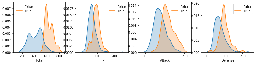
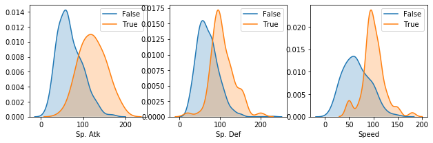
Density plots

Same applies to density plots (if no arguments are passed, all numerical features are considered)

pokemon.plot_density()

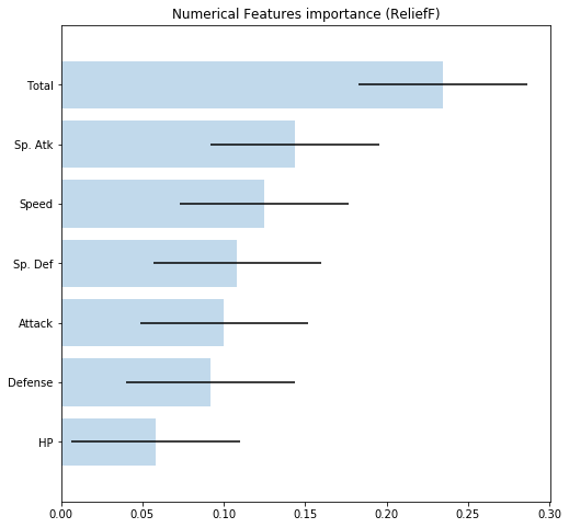
Features importance

To extract features importance, Dataset uses the ReliefF algorithm. By calling the method features_importance() you obtain a Python dictionary with the name of every feature and its relative importance to predict the target variable.

pokemon.features_importance()

{'HP': 0.05809940944881894,
 'Defense': 0.0918786111111111,
 'Attack': 0.10025405405405405,
 'Sp. Def': 0.10831636904761896,
 'Speed': 0.12509607142857132,
 'Sp. Atk': 0.14393648097826098,
 'Total': 0.23443208333333318}

If you want to plot features importance, call plot_importance():

pokemon.plot_importance()

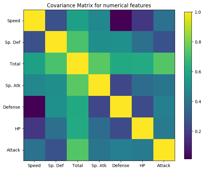
Covariance Matrix

Another useful plot is the covariance matrix. This time, Dataset library adds an interesting and convenient functionality, which is, grouping features with similar covariance together in the same plot. To do so, it uses a hierarchical dendogram to determine what is the best possible order to reflect affinities between features.

To use it, simply type the following:

pokemon.plot_covariance()

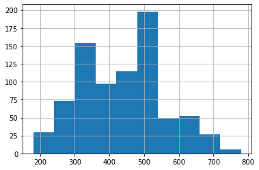
Native pandas plots

In case you want to access native pandas plotting functions, remeber that you can access the entire dataframe by simply accessing the property .features, and from there, you can reference individual variables by its names. From that point, in order to access native pandas hist() for the feature Total, we use:

pokemon.features.Total.hist()

<matplotlib.axes._subplots.AxesSubplot at 0x129bcfe50>

Data cleaning

 NA’s

Identify and remove NA’s is one of the basic capabilities in pandas. To ease that step, Dataset gives you info about features that contain NA’s in the describe() method. If any, you can ask what features are presenting empty values by:

pokemon.nas()

['Type 2']

and remove them, to check that everything worked fine (no need to say what features to fix).

pokemon.drop_na()
pokemon.nas()      # <- this should return an empty array

[]

Replace NA

If you want to replace NA instead of removing, use replace_na().

Outliers

To identify outliers, you can use the method outliers(). You can specify how many neighbours to consider when evaluating if a sample is an outlier (default value is 20). The method will tell you what indices in the dataset contain samples that might be outliers. From this point is your decision to remove them or not, and properly evaluate the effect of that eventual removal.

pokemon.outliers()

array([ 11,  20,  42,  49,  54, 105, 106, 110, 377])

pokemon.drop_samples(pokemon.outliers())

<dataset.dataset.Dataset at 0x10e75a220>

Correlation

Besides all the correlogram capabilities provided by scikit-learn and many other libraries, Dataset simply allows you to compute what is the correlation between features. No plot added, but all the relevant information is returned in a single call. The relevant parameter here is the threshold used to determine whether two features are correlated or not.

pokemon.correlated(threshold=0.7)

[('Total', 'Sp. Atk', 0.7448157606316953),
 ('Total', 'Sp. Def', 0.7409062430885279),
 ('Total', 'Attack', 0.7370599898479868),
 ('Total', 'HP', 0.7224040324193493)]

If you want to consider correlation with the target variable, you should unset the target variable (returning it back to the list of features) to compute its correlation with the remaining features (of the same type).

pokemon.unset_target().to_categorical('Legendary').categorical_correlated(threshold=0.1)

[('Generation', 'Type 2', 0.2806336628669287),
 ('Type 2', 'Legendary', 0.26714501722584993),
 ('Type 1', 'Type 2', 0.24543264607050674),
 ('Generation', 'Type 1', 0.23603346946402512),
 ('Type 1', 'Legendary', 0.19440503723011787),
 ('Generation', 'Legendary', 0.1889106739606925)]

pokemon.set_target('Legendary');

Under represented features

Dataset has a method to see if the values of some of the features are under represented. This situation occurs when one or several possible values from a feature are only present in a residual number of samples.

To discover if your dataset presents this anomaly, simply type:

pokemon.under_represented_features()

[]

which in our case returns an empty array.

 Merge categories

In our case we don’t have that situation. If that would be the case we can merge all under-represented categories together to have a balanced representation of all of them. To do so, we use

my_data.merge_categories(column='color', old_values=['grey', 'black'], new_value='dark')

to fusion values grey and black into a new category dark.

Merge values

If we want to fusion values from numerical features, we should use:

my_data.merge_values(column='years', old_values=['2001', '2002'], new_value='2000')

Data transformation

 One-hot encoding

Some categorical features are better transformed into numerical by performing a one-hot encoding. To do so, we call the method onehot_encode() specifying the list of features we want to convert. If no name is given, then all categorical variables are onehot-encoded.

In this case, the feature called Generation has been previously converted from numerical to categorical, but now we’re transforming it into a dummified version, which will produce 6 new variables called Generation_1 to Generation_6.

pokemon.onehot_encode('Generation').summary()

Features Summary (all):
'Attack'      : float64    Min.(20.0) 1stQ(60.0) Med.(80.0) Mean(83.0) 3rdQ(103.) Max.(190.)
'Defense'     : float64    Min.(15.0) 1stQ(55.0) Med.(75.0) Mean(78.2) 3rdQ(100.) Max.(180.)
'HP'          : float64    Min.(1.0) 1stQ(55.0) Med.(70.0) Mean(70.7) 3rdQ(85.0) Max.(150.)
'Name'        : object     405 categs. 'Bulbasaur'(1, 0.0025) 'Ivysaur'(1, 0.0025) 'Venusaur'(1, 0.0025) 'VenusaurMega Venusaur'(1, 0.0025) ...
'Sp. Atk'     : float64    Min.(20.0) 1stQ(50.0) Med.(70.0) Mean(77.3) 3rdQ(100.) Max.(180.)
'Sp. Def'     : float64    Min.(20.0) 1stQ(55.0) Med.(75.0) Mean(75.4) 3rdQ(95.0) Max.(154.)
'Speed'       : float64    Min.(10.0) 1stQ(50.0) Med.(70.0) Mean(70.9) 3rdQ(92.0) Max.(160.)
'Total'       : float64    Min.(190.) 1stQ(352.) Med.(474.) Mean(455.) 3rdQ(530.) Max.(780.)
'Type 1'      : object     18 categs. 'Grass'(51, 0.1259) 'Fire'(50, 0.1235) 'Bug'(37, 0.0914) 'Normal'(36, 0.0889) ...
'Type 2'      : object     18 categs. 'Poison'(97, 0.2395) 'Flying'(33, 0.0815) 'Dragon'(32, 0.0790) 'Ground'(32, 0.0790) ...
'Generation_1': float64    Min.(0.0) 1stQ(0.0) Med.(0.0) Mean(0.18) 3rdQ(0.0) Max.(1.0)
'Generation_2': float64    Min.(0.0) 1stQ(0.0) Med.(0.0) Mean(0.12) 3rdQ(0.0) Max.(1.0)
'Generation_3': float64    Min.(0.0) 1stQ(0.0) Med.(0.0) Mean(0.20) 3rdQ(0.0) Max.(1.0)
'Generation_4': float64    Min.(0.0) 1stQ(0.0) Med.(0.0) Mean(0.16) 3rdQ(0.0) Max.(1.0)
'Generation_5': float64    Min.(0.0) 1stQ(0.0) Med.(0.0) Mean(0.20) 3rdQ(0.0) Max.(1.0)
'Generation_6': float64    Min.(0.0) 1stQ(0.0) Med.(0.0) Mean(0.12) 3rdQ(0.0) Max.(1.0)
'Legendary'   : object     2 categs. 'False'(394, 0.9728) 'True'(11, 0.0272)

Discretize

In some other ocassions what we need is to transform a numerical variable into a category by discretizing it, o binning. To illustrate this we will transform a numerical variable into a category by specifying ranges of values or bins to consider.

For example, the feature Speed (ranges between 10 and 160) could be discretized by considering only ranges, as follows:

pokemon.discretize('Speed', [(10, 60),(60, 110),(110, 150)],
                   category_names=['low', 'mid', 'high']).summary()

Features Summary (all):
'Attack'      : float64    Min.(20.0) 1stQ(60.0) Med.(80.0) Mean(83.0) 3rdQ(103.) Max.(190.)
'Defense'     : float64    Min.(15.0) 1stQ(55.0) Med.(75.0) Mean(78.2) 3rdQ(100.) Max.(180.)
'HP'          : float64    Min.(1.0) 1stQ(55.0) Med.(70.0) Mean(70.7) 3rdQ(85.0) Max.(150.)
'Name'        : object     405 categs. 'Bulbasaur'(1, 0.0025) 'Ivysaur'(1, 0.0025) 'Venusaur'(1, 0.0025) 'VenusaurMega Venusaur'(1, 0.0025) ...
'Sp. Atk'     : float64    Min.(20.0) 1stQ(50.0) Med.(70.0) Mean(77.3) 3rdQ(100.) Max.(180.)
'Sp. Def'     : float64    Min.(20.0) 1stQ(55.0) Med.(75.0) Mean(75.4) 3rdQ(95.0) Max.(154.)
'Speed'       : category   3 categs. 'low'(212, 0.5261) 'mid'(165, 0.4094) 'high'(26, 0.0645)
'Total'       : float64    Min.(190.) 1stQ(352.) Med.(474.) Mean(455.) 3rdQ(530.) Max.(780.)
'Type 1'      : object     18 categs. 'Grass'(51, 0.1259) 'Fire'(50, 0.1235) 'Bug'(37, 0.0914) 'Normal'(36, 0.0889) ...
'Type 2'      : object     18 categs. 'Poison'(97, 0.2395) 'Flying'(33, 0.0815) 'Dragon'(32, 0.0790) 'Ground'(32, 0.0790) ...
'Generation_1': float64    Min.(0.0) 1stQ(0.0) Med.(0.0) Mean(0.18) 3rdQ(0.0) Max.(1.0)
'Generation_2': float64    Min.(0.0) 1stQ(0.0) Med.(0.0) Mean(0.12) 3rdQ(0.0) Max.(1.0)
'Generation_3': float64    Min.(0.0) 1stQ(0.0) Med.(0.0) Mean(0.20) 3rdQ(0.0) Max.(1.0)
'Generation_4': float64    Min.(0.0) 1stQ(0.0) Med.(0.0) Mean(0.16) 3rdQ(0.0) Max.(1.0)
'Generation_5': float64    Min.(0.0) 1stQ(0.0) Med.(0.0) Mean(0.20) 3rdQ(0.0) Max.(1.0)
'Generation_6': float64    Min.(0.0) 1stQ(0.0) Med.(0.0) Mean(0.12) 3rdQ(0.0) Max.(1.0)
'Legendary'   : object     2 categs. 'False'(394, 0.9728) 'True'(11, 0.0272)

Skewness

Another possibility is to fix the skewness of all those features who could present it. We can do it at once by simply calling fix_skewness(), or if we previously want to check what features present skewness, we can also call skewed_features().

Let’s apply it, first to know what features present skewness (if any):

pokemon.skewed_features()

Generation_6    2.324424
Generation_2    2.221659
Generation_4    1.800833
Generation_1    1.663678
Generation_3    1.480842
Generation_5    1.480842
Sp. Atk         0.673112
Attack          0.533859
HP              0.498398
Defense         0.471578
Sp. Def         0.438338
Total           0.070545
dtype: float64

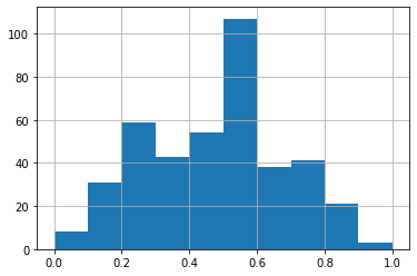
Let’s fix skewness and plot the historgram before and after in the same plot.

plt.figure(figsize=(8,3))
plt.subplot(121)
pokemon.features['HP'].hist()

# Fix skewness
pokemon.fix_skewness()

plt.subplot(122)
pokemon.features['HP'].hist()
plt.show()

Scale

It depends on the method that you use, but it is normally accepted that scaling your numeric features is a good practice. If you want to do so, you can easily do it by calling:

pokemon.scale(method='MinMaxScaler')

<dataset.dataset.Dataset at 0x10e75a220>

If you don’t specify any parameters, scaling will be applied to numerical features, and the method will return the dataset with those features already scaled using StandardScaler. But you can also specify MinMaxScaler as method, if you want a different scaling method to be applied. The result is that numerical features range now between 0 and 1.

To confirm that scaling worked properly let’s plot the histogram of the feature Totals, to see that the X-axis is now ranging between 0 and 1, instead of 0 and 800, as in the previous section plot.

pokemon.features.Total.hist()

<matplotlib.axes._subplots.AxesSubplot at 0x1297c5df0>

Speed is now a category that only presents three possible values (whose labels have been provided).

Feature selection

Information Gain

To compute the information gain provided by each categorical feature with respect to the target variable (must be set) then, you can use the method information_gain(). The result is a dictionary with key-value pairs, where each key corresponds to the categorical variables, and the value is the IG:

ig = pokemon.information_gain()

for k in ig:
    print('{:<7}: {:.2f}'.format(k, ig[k]))

Name   : 0.18
Speed  : 0.00
Type 1 : 0.04
Type 2 : 0.03

From this info, it could be safe to remove the variable Speed, but must always test your hypothesis first.

Stepwise feature selection

We can force a feature selection process with our features by calling stepwise_selection(). We must be sure that the features used in the selection process are all numerical. If that is not the case, call onehot_encode() before using this method.

In our case, we must adapat a little bit our problem to suit the needs of stepwise_selection(). We need target variable to be numeric. To achieve that, we must unset the target variable Legendary in order to bring it back list of features. Then we call the method onehot_encode() (only works over the features, not the target variable), and then set the target again.

Remember that we can chain method calls:

pokemon.unset_target()
pokemon.onehot_encode('Legendary').drop_columns('Legendary_False')
pokemon.set_target('Legendary_True').summary()

Features Summary (all):
'Attack'        : float64    Min.(0.0) 1stQ(0.36) Med.(0.48) Mean(0.48) 3rdQ(0.61) Max.(1.0)
'Defense'       : float64    Min.(0.0) 1stQ(0.37) Med.(0.50) Mean(0.50) 3rdQ(0.64) Max.(1.0)
'Generation_1'  : float64    Min.(0.0) 1stQ(0.0) Med.(0.0) Mean(0.18) 3rdQ(0.0) Max.(1.0)
'Generation_2'  : float64    Min.(0.0) 1stQ(0.0) Med.(0.0) Mean(0.12) 3rdQ(0.0) Max.(0.99)
'Generation_3'  : float64    Min.(0.0) 1stQ(0.0) Med.(0.0) Mean(0.20) 3rdQ(0.0) Max.(1.0)
'Generation_4'  : float64    Min.(0.0) 1stQ(0.0) Med.(0.0) Mean(0.16) 3rdQ(0.0) Max.(1.0)
'Generation_5'  : float64    Min.(0.0) 1stQ(0.0) Med.(0.0) Mean(0.20) 3rdQ(0.0) Max.(1.0)
'Generation_6'  : float64    Min.(0.0) 1stQ(0.0) Med.(0.0) Mean(0.12) 3rdQ(0.0) Max.(0.99)
'HP'            : float64    Min.(0.0) 1stQ(0.49) Med.(0.58) Mean(0.58) 3rdQ(0.67) Max.(0.99)
'Name'          : object     403 categs. 'Bulbasaur'(1, 0.0025) 'Ivysaur'(1, 0.0025) 'Venusaur'(1, 0.0025) 'VenusaurMega Venusaur'(1, 0.0025) ...
'Sp. Atk'       : float64    Min.(0.0) 1stQ(0.37) Med.(0.51) Mean(0.52) 3rdQ(0.68) Max.(1.0)
'Sp. Def'       : float64    Min.(0.0) 1stQ(0.37) Med.(0.52) Mean(0.51) 3rdQ(0.66) Max.(1.0)
'Speed'         : category   3 categs. 'low'(212, 0.5261) 'mid'(165, 0.4094) 'high'(26, 0.0645)
'Total'         : float64    Min.(0.0) 1stQ(0.30) Med.(0.51) Mean(0.47) 3rdQ(0.60) Max.(1.0)
'Type 1'        : object     18 categs. 'Grass'(51, 0.1266) 'Fire'(49, 0.1216) 'Bug'(36, 0.0893) 'Normal'(36, 0.0893) ...
'Type 2'        : object     18 categs. 'Poison'(96, 0.2382) 'Flying'(33, 0.0819) 'Dragon'(32, 0.0794) 'Ground'(32, 0.0794) ...
'Legendary_True': float64    Min.(0.0) 1stQ(0.0) Med.(0.0) Mean(0.02) 3rdQ(0.0) Max.(1.0)

We remove then the column called Legendary_False as the column Legendary_True already behaves numerically as we want (0.0 means False, and 1.0 means True).

Now, we let the stepwise algorithm to decide what features could be safe to remove:

pokemon.stepwise_selection()

Considering only numerical features

['Generation_3', 'Generation_4']

In a one-liner, we drop the columns/features selected by the stepwise algorithm and then printout the summary.

pokemon.drop_columns(pokemon.stepwise_selection()).summary()

Considering only numerical features
Features Summary (all):
'Attack'        : float64    Min.(0.0) 1stQ(0.36) Med.(0.48) Mean(0.48) 3rdQ(0.61) Max.(1.0)
'Defense'       : float64    Min.(0.0) 1stQ(0.37) Med.(0.50) Mean(0.50) 3rdQ(0.64) Max.(1.0)
'Generation_1'  : float64    Min.(0.0) 1stQ(0.0) Med.(0.0) Mean(0.18) 3rdQ(0.0) Max.(1.0)
'Generation_2'  : float64    Min.(0.0) 1stQ(0.0) Med.(0.0) Mean(0.12) 3rdQ(0.0) Max.(0.99)
'Generation_5'  : float64    Min.(0.0) 1stQ(0.0) Med.(0.0) Mean(0.20) 3rdQ(0.0) Max.(1.0)
'Generation_6'  : float64    Min.(0.0) 1stQ(0.0) Med.(0.0) Mean(0.12) 3rdQ(0.0) Max.(0.99)
'HP'            : float64    Min.(0.0) 1stQ(0.49) Med.(0.58) Mean(0.58) 3rdQ(0.67) Max.(0.99)
'Name'          : object     403 categs. 'Bulbasaur'(1, 0.0025) 'Ivysaur'(1, 0.0025) 'Venusaur'(1, 0.0025) 'VenusaurMega Venusaur'(1, 0.0025) ...
'Sp. Atk'       : float64    Min.(0.0) 1stQ(0.37) Med.(0.51) Mean(0.52) 3rdQ(0.68) Max.(1.0)
'Sp. Def'       : float64    Min.(0.0) 1stQ(0.37) Med.(0.52) Mean(0.51) 3rdQ(0.66) Max.(1.0)
'Speed'         : category   3 categs. 'low'(212, 0.5261) 'mid'(165, 0.4094) 'high'(26, 0.0645)
'Total'         : float64    Min.(0.0) 1stQ(0.30) Med.(0.51) Mean(0.47) 3rdQ(0.60) Max.(1.0)
'Type 1'        : object     18 categs. 'Grass'(51, 0.1266) 'Fire'(49, 0.1216) 'Bug'(36, 0.0893) 'Normal'(36, 0.0893) ...
'Type 2'        : object     18 categs. 'Poison'(96, 0.2382) 'Flying'(33, 0.0819) 'Dragon'(32, 0.0794) 'Ground'(32, 0.0794) ...
'Legendary_True': float64    Min.(0.0) 1stQ(0.0) Med.(0.0) Mean(0.02) 3rdQ(0.0) Max.(1.0)

Dataset Split

Dataset adds a method to split your dataset according to the specified proportions between training and test. The method is called split(), and accepts as optional parameter the percentage to be assigned to the test set.

We normally split specifying the seed used by the random number generator. If you plan to repeat the split process a number of times within a CV process, you need to change the seed accordingly.

X, y = pokemon.split(seed=1)

What we obtain in X and y, are two objects that inside contain the training and test splits, as pandas DataFrames. To access them, we simply write:

X.train
X.test
y.train
y.test

Let’s check it out:

X.train.head(3)

	Attack	Defense	Generation_1	Generation_2	Generation_5	Generation_6	HP	Name	Sp. Atk	Sp. Def	Speed	Total	Type 1	Type 2
185	0.575444	0.335548	0.0	0.0	0.0	0.0	0.426154	Anorith	0.265005	0.328587	mid	0.309899	Rock	Bug
227	0.778264	0.611023	0.0	0.0	0.0	0.0	0.556204	LopunnyMega Lopunny	0.393294	0.672391	high	0.688447	Normal	Fighting
245	0.633856	0.439686	0.0	0.0	0.0	0.0	0.661813	Toxicroak	0.609585	0.453749	mid	0.541394	Poison	Fighting

y.test.head(3)

	Legendary_True
360	0.0
62	0.0
374	0.0

Depending on the ML method used, you can directly pass X.train and y.train as DataFrames, or in some other cases to you need to pass the numpy array of values. In that case you simple use:

X.train.values, y.train.values

Same applies to test subsets.